Analyzing the Correlation between Swing Speed and Related Metrics in Major League Baseball
R
mlb
Authors
Atticus Renault
Noah Tobias
Sean Dasovich
Published
May 2, 2025
Introduction
Tracking statistics has been a core part of baseball since its birth in the 19th century. What began as tabulating hits and runs has evolved into batting averages, on base percentages, and complex measures of a player’s “win contribution”. The 2011 movie Moneyball, based on the Oakland Athletics 2002 season, brought advanced metrics to the public’s eye and revealed statistics as a core component to gaining a competitive edge. This hyper-analysis of player performance is commonly referred to today as “sabermetrics”. One of the key stats that emerged out of the data revolution was bat speed. The basic principle that “the harder you swing, the farther the ball goes” has become increasingly valuable in the modern game, which emphasizes home runs and big hits. This paper explores the relationship between bat speed and other metrics, assessing its advantages and trade-offs.
In this project, we explore three core research questions:
Does a batter’s primary position affect his batting performance?
Does the league a batter plays in affect his batting performance?
What factors (e.g., home runs, whiff %, strikeout %, hard hit %, average launch angle) are most influenced by bat speed for Major League Baseball batters?
These questions aim to understand bat speed’s place in baseball today and the role of external factors in affecting a batter’s approach/training. The insights from this data analysis could influence multiple levels of the baseball pipeline. At the training stage, these results may reveal how valuable bat speed is as a trainable skill. When thinking about primary position, these findings could result in further discussion about balancing defensive and offensive proficiency. At a structural level, our analysis can be used in determining if the National and American leagues value different attributes in a player.
Data Provenance
For this project, we used two datasets. The primary dataset is most helpful in addressing the first research question and sets the foundation for the data analysis. The second dataset provides a new perspective on this topic through a categorical lens. The two datasets were combined through data wrangling and cleaning processes to produce a final dataset for analysis.
Description: Baseball Savant, powered by Statcast MLB, allows for customized data tables which can then be converted to csv files (Baseball Savant 2024). We created a custom table that includes all qualified (at least 502 plate appearances) batters from the 2024 regular season. Our custom table includes 19 columns and 129 rows.
Purpose: This dataset was used to gather bat speed and related attributes for MLB batters from the 2024 regular season. The information in this table was useful for determining correlation between bat speed and the other commonly collected baseball statistics (hard hit %, strikeout %, etc.)
Cases: Each row represents an MLB batter, with columns describing various batting statistics.
Description: Baseball Reference is part of an independent encyclopedia of sports statistics (Baseball Reference 2024). It provides a lot of the same information as Baseball Savant but is better for finding individual player information. Baseball Reference also has tables of aggregate season data from which we could find batters’ league (American or National) and primary position (infield, outfield, or DH). The original table for 2024 has 34 columns and 741 rows.
Purpose: This dataset was used to collect the league designation (AL or NL) and primary position for each MLB player in the 2024 regular season. This information is used to group players in data visualizations by common characteristics.
Cases: Each row represents an MLB player, not necessarily batter, who made an appearance in 2024 with the columns describing various batting statistics.
Exploratory Data Analysis (EDA)
Our exploratory data analysis includes a summary table with descriptive statistics for the population of interest (qualified MLB batters). Additionally, we created various other data visualizations to examine relationships between relevant statistics. These tables and visualizations were used to draw conclusions regarding trends in player performance.
We started by constructing summary tables to provide an overview of key statistics such as runs, boundaries, batting average, strike rate, and more. These tables allowed us to compare metrics across players and batting styles, highlighting trends and differences in performance.
Next, we developed data visualizations to explore deeper relationships and distributions within the dataset:
Scatter plots: These helped us visualize how variables like runs, boundaries, balls faced, matches, batting average, batting strike rate, and boundaries percentage relate to batting strike rate, with batting styles distinguished by color.
Correlation heatmap: This highlighted the strength of relationships between batting strike rate and other performance metrics.
Bar graphs: These graphs compared the two leagues, American and National, on the average of their players’ average swing speed and the total home runs hit. (Note that a few players played in both leagues during that year; they were put into their own category).
The insights gained from these analyses form the foundation of our results and conclusions. Below, we detail the most critical tables and visualizations, along with the key insights they helped us derive.
Batting Metrics Summary Table
Table 1 provides a baseline for the level we can expect from these MLB players. While these summary statistics alone are not particularly enlightening, they set the background for future comparison.
Table 1: Summary Statistics for Key Batting Variables
Variable
Mean
Median
Minimum
Maximum
Home Run
21.67
20.0
2.0
58.0
Walk
53.50
52.0
15.0
133.0
K %
21.06
21.1
4.3
34.4
Intentional Walk
2.64
2.0
0.0
20.0
Avg Swing Speed (mph)
71.92
71.8
63.1
78.6
Avg Launch Angle
13.60
13.7
4.0
24.4
Hard Hit %
41.85
41.7
19.5
61.0
Whiff %
24.05
24.4
6.9
36.4
Key Insights:
In general, the mean is close to the median, which indicates that there are not significant skews in either direction.
Over the course of a season, the average player – playing most regular season games – hits about 22 home runs and walks about 57 times (3 of which are intentional).
That same player has an average bat speed of 72 mph, launching the ball around 14 degrees (above the plane parallel to the ground) and missing the ball 24% of the time.
When making contact, that player can expect a hard hit ball (exit velocity of 95+ mph) about 42% of the time.
Factors Influenced by Average Bat Speed
Our analysis of bat speed continues with closer look at potential correlations between bat speed and other metrics. Specifically, the following section contains two scatterplots: one comparing bat speed to home runs and the other comparing bat speed to strikeout %. These visuals are followed up by a correlation heatmap which displays correlations between metrics broadly.
Scatter Plots
Figure 1 visualizes the correlation between average bat speed (interchangeable with average swing speed) and home runs hit by qualified MLB batters. Home runs are increasingly emphasized in modern baseball, so this scatterplot could shed some light on how these metrics are related.
Figure 1
Key Insights:
There is a moderate, positive correlation between average swing speed and home runs hit by qualified MLB batters.
The biggest cluster is around a swing speed in the low 70s and around 20 home runs.
In case you were wondering, the two 2024 MVPs, Aaron Judge and Shohei Ohtani, are the two cases with the most home runs (though not the highest average swing speed).
Figure 2 is another scatterplot, this time comparing average swing speed with a batter’s strikeout % (the percent of plate appearances the result in a strikeout). With more emphasis on bigger hits, this visualization can determine if there is a trade-off required.
Figure 2
Key Insights:
There is a slight positive correlation between average swing speed and strikeout % but the points are more spread out than in the previous scatterplot. Overall, there seems to be somewhat of a trade-off for increasing bat speed.
A significant factor not captured by this plot is a batter’s “plate discipline”, essentially how likely they are to swing at bad pitches. Batter’s with high swing speed are not necessarily less selective than batter’s with low swing speed.
However, a slower swing does keep the bat in the strike zone for longer, increasing the chances of making contact, even on a bad pitch. This could explain why the correlation is more defined at the lower end of the bottom axis.
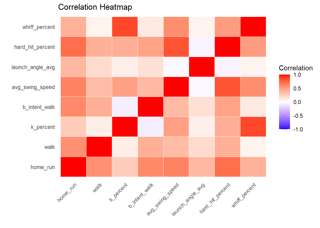
Correlation Heatmap
Figure 3 shows the relative strength of how each batting statistics influences every other statistic. The diagonal will be perfect correlation, and the matrix as a whole is symmetric since metrics are mirrored on either axis.
Figure 3
Key Insights:
Apart from the one-to-one correlations, the strongest correlations between attributes are between strikeout % and whiff % and also between average swing speed and hard hit %.
The areas of little to no correlation are between strikeout % and intentional walks, average launch angle and average swing speed, and hard hit % and average launch angle. This is interesting considering average launch angle is a metric commonly associated with home runs, though too high of a launch angle will result in a pop-up.
There are no negative correlations between variables; they all generally increase with respect to each other.
Influence of League and Position
Now that we have examined relationships between batting metrics, we will expand our analysis to categorical factors: league and position. It’s worth noting that the National League adopted the DH only as recently as 2022 (before that, pitchers hit). The following bar graphs and scatterplots may reveal any remnants of pitcher-lowered average bat speed.
Bar Graphs
Figure 4 breaks down average swing speed by league. The “2LG” category is players who played in both leagues in 2024. The sample size for that is only 5, so it is not statistically significant.
Figure 4
Key Insights:
The average of each league’s batter’s average swing speed is approximately the same. There is essentially no difference between the leagues as far as swing speed is concerned.
For both leagues, the average swing speed was a little over 70 mph. This is very similar to the overall MLB average swing speed of 71.92 mph found in Table 1.
Figure 5 looks at the average number of home runs hit per batter in the American and National Leagues.
Figure 5
Key Insights:
Like the previous graph, there is little difference between the American League and National League with regard to the average per player home runs hit.
The American League has a slight edge but both leagues rest around 22 home runs per player. This is similar to the MLB-wide average of 21.67 in Table 1.
League does not appear to be an indicator of a batter’s home run production.
Scatterplot
Figure 6 displays a visualization divided into the three league designations with points plotted by walks and home runs. The points are color coded by the primary position of the MLB player.
Figure 6
Key Insights:
In terms of the correlation between walks and home runs, both leagues exhibit a moderate positive relationship.
The AL and NL distributions have similar shapes with each having high potential outliers. The National League distribution does have a few more players with low home run counts but is also densely populated around the average of the dataset.
The positions “Infielder” and “Outfielder” are evenly dispersed in terms of walks, but there tends to be more infielders on the higher end of home runs. It’s worth noting that there are more infielders than outfielders by virtue of the layout of a baseball field.
While there are not enough DHs to be significant, it is interesting to note that the National League’s potential upper outliers are all DHs, and the American League’s potential upper outliers are all outfielders.
Conclusion
Concerning bat speed’s influence on other metrics for qualified MLB batters in the 2024 season, there are positive correlations between bat speed and home runs (Figure 1) and bat speed and strikeout % (Figure 2). The distribution for bat speed vs. strikeout %, however, is more spread, indicating a weaker correlation. Figure 3 explores more correlations concerning bat speed and additionally distinguishes the relationships between other batting metrics. Notable positive correlations include those between strikeout % and whiff % as well as between average swing speed and hard hit %.
With respect to league and primary position for qualified batters in the 2024 MLB season, there is no relationship between the a batter’s league and his average bat speed or a batter’s league and his average home runs as displayed by Figure 4 and Figure 5.
Additionally, Figure 6 indicates that there is not a relationship between walks and the position one plays. There may be a relation between position and home runs hit, but the sample size might need to be expanded before making that conclusion.
Code Appendix
Code
## Load Necessary Packageslibrary(tidyverse)library(dplyr)library(knitr)library(kableExtra)library(reshape2)library(ggplot2)# Step 1: Read CSV without column namesmlb_data_raw <-read_csv("https://raw.githubusercontent.com/nwt5144/FinalProjectStat184/refs/heads/main/stats.csv", show_col_types =FALSE)# Create Summary Statistics Table ----batting_data <- mlb_data_raw %>%select('last_name, first_name', home_run, walk, k_percent, b_intent_walk, avg_swing_speed, launch_angle_avg, hard_hit_percent, whiff_percent )# Calculate summary statisticssummary_table <- batting_data %>%reframe(Variable =c("home_run", "walk", "k_percent", "b_intent_walk", "avg_swing_speed", "launch_angle_avg","hard_hit_percent","whiff_percent" ),Mean =c(mean(home_run, na.rm =TRUE), mean(walk, na.rm =TRUE), mean(k_percent, na.rm =TRUE), mean(b_intent_walk, na.rm =TRUE), mean(avg_swing_speed, na.rm =TRUE), mean(launch_angle_avg, na.rm =TRUE),mean(hard_hit_percent, na.rm =TRUE), mean(whiff_percent, na.rm =TRUE) ),Median =c(median(home_run, na.rm =TRUE), median(walk, na.rm =TRUE), median(k_percent, na.rm =TRUE), median(b_intent_walk, na.rm =TRUE), median(avg_swing_speed, na.rm =TRUE), median(launch_angle_avg, na.rm =TRUE),median(hard_hit_percent, na.rm =TRUE), median(whiff_percent, na.rm =TRUE) ),Minimum =c(min(home_run, na.rm =TRUE), min(walk, na.rm =TRUE), min(k_percent, na.rm =TRUE), min(b_intent_walk, na.rm =TRUE), min(avg_swing_speed, na.rm =TRUE), min(launch_angle_avg, na.rm =TRUE),min(hard_hit_percent, na.rm =TRUE), min(whiff_percent, na.rm =TRUE) ),Maximum =c(max(home_run, na.rm =TRUE), max(walk, na.rm =TRUE), max(k_percent, na.rm =TRUE), max(b_intent_walk, na.rm =TRUE), max(avg_swing_speed, na.rm =TRUE), max(launch_angle_avg, na.rm =TRUE),max(hard_hit_percent, na.rm =TRUE), max(whiff_percent, na.rm =TRUE) ) )# Display Summary Statistics Table ----summary_table %>%kable(caption ="Summary Statistics for Key Batting Variables", digits =2, align =c("l", rep("c", 4)) ) %>%kable_styling(bootstrap_options =c("striped", "hover", "condensed"), full_width =FALSE, font_size =14 ) %>%row_spec(0, bold =TRUE) # Bold header row# Prepare batting_data for mergingbatting_data_for_combo <- batting_data %>%separate(`last_name, first_name`, into =c("LastName", "FirstName"), sep =", ", remove =FALSE) %>%select(-`last_name, first_name`) %>%mutate(Player =paste(FirstName, LastName),Player =str_trim(Player) )# Read roster dataroster_data <-read_csv("https://raw.githubusercontent.com/nwt5144/FinalProjectStat184/refs/heads/main/NlAlPos.csv")# Clean roster_dataroster_data1 <- roster_data %>%mutate(Player =str_replace(Player, "\\*", ""), Player =str_trim(Player) ) roster_data2 <- roster_data1 %>%mutate(Player =str_replace(Player, "\\#", ""), Player =str_trim(Player) )roster_data3 <- roster_data2 %>%mutate(Pos =str_replace(Pos, "\\*", ""), Pos =str_trim(Pos) )roster_data4 <- roster_data3 %>%distinct(Player, .keep_all =TRUE)# Keep only necessary columnsroster_data_small <- roster_data4 %>%select(Player, Lg, Pos)# Merge on Playercombined_data <- batting_data_for_combo %>%left_join(roster_data_small, by ="Player")# Clean and group Poscombined_data <- combined_data %>%mutate(Pos =str_replace_all(Pos, "\\*", ""),Pos =str_extract(Pos, "."),Pos =case_when( Pos =="1"~"Pitcher", Pos %in%c("2", "3", "4", "5", "6") ~"Infielder", Pos %in%c("7", "8", "9") ~"Outfielder", Pos =="D"~"DH",TRUE~NA_character_ ) )head(combined_data)# Scatterplot: Home Run vs Average Swing Speedggplot(batting_data, aes(x = avg_swing_speed, y = home_run)) +geom_point(color ="blue", alpha =1) +labs(title ="Home Runs vs Average Swing Speed (mph)",x ="Average Swing Speed (mph)",y ="Home Runs" ) +theme_minimal()# Scatterplot: K% vs Hard Hit %ggplot(batting_data, aes(x = avg_swing_speed, y = k_percent)) +geom_point(color ="red", alpha =1) +labs(title ="Strikeout Percentage vs Average Swing Speed (mph)",x ="Average Swing Speed (mph)",y ="Strikeout Percentage" ) +theme_minimal()# raw column namescolumn_names <-c("home_run","walk","k_percent","b_intent_walk","avg_swing_speed","launch_angle_avg","hard_hit_percent","whiff_percent")# map each one to a ‐readable labelfull_names <-setNames(c("Home Runs","Walks","Strikeout Percentage","Intentional Walk Percentage","Average Swing Speed (mph)","Average Launch Angle (°)","Hard-Hit Percentage","Whiff Percentage" ), column_names)# heatmap, swapping in the labelsggplot(correlation_melt, aes(x = Var1, y = Var2, fill = value)) +geom_tile(color ="white") +scale_fill_gradient2(low ="blue",mid ="white",high ="red",midpoint =0,limit =c(-1, 1),space ="Lab",name ="Correlation" ) +scale_x_discrete(labels = full_names) +scale_y_discrete(labels = full_names) +theme_minimal() +theme(axis.text.x =element_text(angle =45, vjust =1, hjust =1) ) +labs(title ="Correlation Heatmap",x =NULL,y =NULL )avg_swing_speed_league <- combined_data%>%group_by(Lg) %>%summarize(avg_swing_speed =mean(avg_swing_speed, na.rm =TRUE))hr_league <- combined_data%>%group_by(Lg) %>%summarize(hr = home_run)# Scatterplot: Home Runs vs Hard Hit % by Position Groupggplot(avg_swing_speed_league, aes(x = Lg, y = avg_swing_speed)) +geom_col() +labs(title ="Average Swing Speed by League",x ="League",y ="Average Swing Speed (mph)" ) +theme_minimal()# Bar Graph: Total Home Runs by Leagueggplot(hr_league, aes(x = Lg, y = hr)) +geom_col() +labs(title ="Total Home Runs by League",x ="League",y ="Home Runs" ) +theme_minimal()# Scatterplot: Home Runs vs Walks by League and Positionggplot(combined_data, aes(x = walk, y = home_run, color = Pos)) +geom_point(alpha =1, size =2) +facet_wrap(~ Lg) +labs(title ="Home Runs vs Walks by League and Position",x ="Walks",y ="Home Runs" ) +theme_minimal()